Three Key Takeaways:
- Renting a home instead of buying can lead to millions more in retirement
- This model can help evaluate the opportunity cost of home ownership versus renting and investing
- Cash flow is critical, reducing your monthly costs and investing the difference will have the most impact on long term net worth
This is part 3 of an article written to demonstrate the incredible power of compound interest, the ability to access that power through the stock market, and how to determine if the stock market is better than home ownership. The ideas herein are complemented with an accompanying dashboard that can be used to enter in assumptions relevant to your situation. Technical people can find my source code on GitHub. Enjoy!
Buying a home
Buying a house is one of the biggest purchases anyone will make in their lifetime. For 30+ years, home ownership has been the centerpiece of the American dream and has been proclaimed as the best way to build wealth. This model may demonstrate otherwise, showing instead that the stock market is the best way to build wealth. This idea has been catching on as millennial move into the phase of home ownership and realize how expensive it can be to buy your first house. Additionally, after 30 years of falling interest rates, can home prices continue increasing at the same rate, especially knowing interest rates cannot go much lower, and may even increase at some point?
This analysis will not review the qualitative aspects of owning a home such as:
- Embedding into a neighborhood and community
- Knowing you won’t have to move after a rental agreement expires
- Having no landlord
- Buying nice things to improve your home
- Putting sweat equity into your home to increase the value
It will also not consider the qualitative aspects of renting (e.g. enhanced flexibility and less liability). Instead this model and analysis is strictly designed to look at the dollar opportunity cost of owning a home versus investing in the stock market.
Calculating Opportunity Cost
To accurately capture opportunity cost, the model was built to consider every factor that might impact the true cost-benefit of home ownership such as maintenance, interest tax deduction, property tax, etc. Three stock market scenarios are run in two parallel tracks of renting and buying. The model invests any monthly cash flow difference into the stock market for the track that incurs the lower monthly cost. .
For example, if your down payment and closing cost is 100,000, then in the rental track the model will invest 100,000 in the stock market. If your rent is 1,000 cheaper per month than your net home ownership cost, this will also be invested in the stock market. If there is a point where monthly rental costs exceed home ownership, then the difference will be invested in the stock market under the home ownership track.
The biggest drivers of the model are the monthly cash flow figures and expected house appreciation value versus the stock market growth expectation. As was highlighted in part 1 and part 2, small investments can compound over time and result in massive differences. This model attempts to identify those small differences to see the true compounding effect that may be lost with home ownership.
This article will look at 4 different scenarios:
- Baseline scenario of 2% annual home appreciation and 9% stock market growth
- Growth scenario of 4% annual home appreciation and 10% stock market growth
- Lower scenario of 1% annual home appreciation and 5% stock market growth
- Baseline scenario 1 (2% and 9%) but using 5% down instead of 20%
Each scenario has the straight line stock market growth (Blue columns) but will also show the actual S&P Total Return over the last 30 years as another comparison point (Green columns).
For simplicity, the model will hold all buyer information constant such as home price, rental cost, maintenance, tax implications, etc. Those assumptions are listed below:
- Home price of $750k with a 30 year fix at 4% with 1.25% property taxes
- Amount down 20% (except scenario 4 where it is 5%)
- Closing costs of 3%
- Comparable rental cost of $3,000 increasing at 2% per year
- Married couple at 40% tax, with a pre mortgage interest tax deduction of $10,000 (SALT max)
- Annual home insurance of $3,500 and annual maintenance of $3,000
Another important caveat is that his model begins calculating at the time of home purchase. It does not consider how the down payment was obtained. If the down payment has been sitting in cash for 5 years then the opportunity cost of the market is potentially greater, but not considered in this model.
The return on investment (ROI) will be calculated by using Internal Rate of Return (IRR). This will consider the time that cash becomes available for investing and calculate the compounding of each individual investment from that time forward. It helps to evaluate two different investments by considering cash availability.
For my analysis, I will site the figures in the blue columns (straight line growth). The green columns are for reference (actual 30 year stock market returns).
Scenario 1: 2 % Annual House Appreciation and 9% Stock market growth
The user defined market expectation of 9% shows only a small divergence out to year 10 at which point the cost savings in renting begin to compound. By year 20, you have $500k+ more by investing in the stock market than by owning a home. By year 30, that divergence has grown to almost $2m!
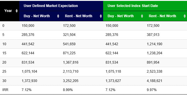
Figure 1: Scenario 1 - Rent 3,000 with 9% annual return
As they say, cash is king! It is important to consider your monthly payments. While the monthly rental cost is only 3,000 in year 1, the net mortgage monthly cost after all expenses and tax credits is 3,804. Overtime, your rent will probably increase faster than your ownership payment, but your ownership payment still increases as property taxes rise, maintenance increases, and you lose the interest tax deduction.
Below is a breakdown of the first month, last month, and 360 month total. As a renter, if you are investing the $804 difference then you will magnify your returns.
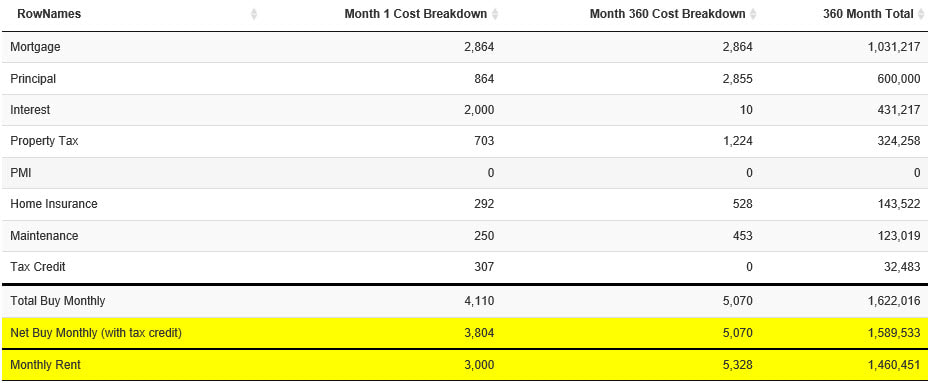
Figure 2: Monthly costs
One important note is that the model does start to favor home ownership if your rent is 4,000. Table 3 shows the impact of paying too much in rent. This highlights that the market is not always better than home ownership, but is very specific to each situation.
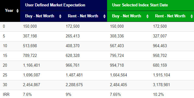
Figure 3: Scenario 1 - Rent 4,000 with 9% annual return
Scenario 2: 4 % Annual House Appreciation and 10% Stock market growth
In this example, we use a 4% annual house appreciation which indicates the house will double in value every 18 years. The change from 2% to 4% results in the buyer having increased their net worth by $1m compared to scenario 1. That being said, the 1% increases in market return from 9% to 10% increases the renters value by $1.4m in year 30, the renter is still far ahead of the buyer, this time by $2.3m. Despite having similar IRR, because renting is cheaper, the small dollar investments each month compound.
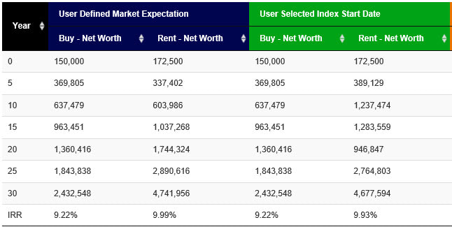
Figure 4: Scenario 2 - Rent 3,000
Scenario 3: 1 % Annual House Appreciation and 5% Stock market growth
While it is always nice to assume high returns, it is important to consider slower growth going forward. The last 30 years have seen a steady trend in falling interest rates that have pushed real estate and stock market growth rates above long term averages. With the world drowning in debt, perhaps our period of high growth has come to an end. If we consider a period of much slower growth, the advantage of renting over buying completely disappears.
In this example, assuming you have a 10+ year time horizon, I would probably pursue home ownership because of the qualitative benefits mentioned in the introduction.
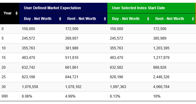
Figure 5: Scenario 3 - Rent 3,000
Scenario 4: 2 % Annual House Appreciation and 9% Stock market growth, 5% down
Saving up for a big down payment is difficult. In these situations you can put down less than 20% but will pay PMI (Private Mortgage Insurance) to protect the lender in the event of a default. With PMI and higher mortgage payments, the monthly net cost rises from 3,804 to 4,636. Down payments and closing costs are certainly more affordable, falling from $172,500 to 60,000 but absorbing an extra 800 a month can be tough on most budgets. Additionally, you lose about 38% your initial investment in closing costs that cannot be recouped, this is why 37,500 is in the buy vs the full 60,000 in the rent scenario.
By putting less down, the leverage ratio has increased significantly. In this scenario, the house appreciation assumption will have a much larger effect on the total net worth. Even so, because you lost so much in closing costs and have such higher monthly payments, the market scenario will still result in a higher net worth at every point in time. The ownership track keeps pace with the market early on due to the 20-1 leverage ratio, but this effect fades as the mortgage is paid down.
Pleases note: You can also pursue a second mortgage rather than PMI but this is not modeled here.
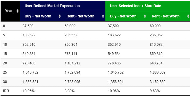
Figure 6: Scenario 4
As can be seen below, net monthly payments have increased substantially by only putting 5% down. Cash flow is very important and should always be considered before locking into a high monthly payment for a relatively illiquid asset.
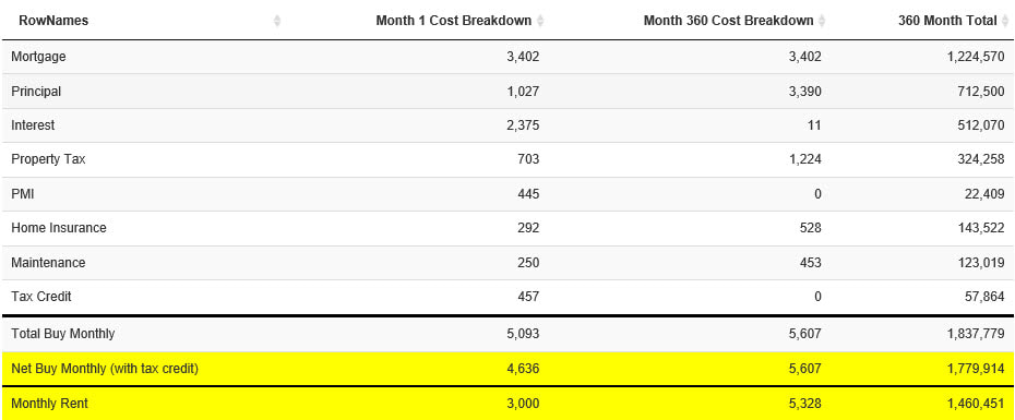
Figure 7: Scenario 4 - Monthly Costs
Wrapping up
The bottom line is to keep your monthly costs as small as possible to improve cash flow. The model will generally show that whichever course has better cash flow will result in a higher net worth assuming you invest the difference. The ideal situation is locking into a low monthly fixed mortgage, but in many markets, monthly rent is less costly than a mortgage. Additionally, the tax benefit of home ownership is not nearly as advantageous after the 2017 tax law nearly doubled the standard deduction while also capping the interest deduction at 750k.
A model is only as good as the inputs (assuming the model is correct to begin with). A good model can guide you in making decisions by evaluating the quantitative differences between scenarios. You can then isolate the qualitative aspects for a holistic analysis.
When using a model, being realistic is critical. A model can be adjusted to create any output. As can be seen above, small changes in assumptions can have huge affects, By changing the rent from 3,000 to 4,000 per month in scenario 1, the model went from favoring renting by $2m to favoring home ownership by $200k. That is a massive difference for a small change in the model. Have fun experimenting, but when making a decision try to find the outcome that is most probable. Anyone can plug in 5% home ownership growth with 4% market returns, but you have to consider the realistic possibility of that outcome. Returns of 4% in the market over 30 years would be a massive deviation to anything that has happened historically, especially if real estate increases at 5% per year.
In this three part series we looked at the power of compound interest, how the stock market provides access to decent rates of return, and how to evaluate the opportunity cost of buying a house. I hope you have gained some insight or can at least use the dashboard to guide you in making some decisions that can have implications far into the future.
Disclosure: The content herein is my own opinion and should not be considered financial
advice or recommendations. I am not receiving compensation for any materials produced.
I have no business relationship with any companies mentioned.